Numerical Methods in Visual Computing – Intro + Part I „Least Squares Optimization“

After several years as junior researcher in diverse disciplines and at diverse institutions working on Visual Methods, I came to the insight that it is not easy to focus one owns reading, research and personal development in Visual Computing. Numerical Methods are a key aspect in the majority of topics and techniques in the field. Although teaching staff members everywhere tend to criticise the mathematical level of interested student, many people underestimate one key aspect: There are so many numerical methods out, available and possibly important to the students – how can we expect beginners in the field to make a good reading selection ? The general will of beginners is to find good selection of methods to learn that covers the large extents and get them the furthest within the field.

Within this blog series, I’d like to propose a base selection of Numerical Methods that are of general nature and that cover a wide range of applications and application disciplines. The selection is meant hereby as a discussion basis for lecturers and interested people in the field of Visual Computing, but it may also serve as inspiration to young researchers to get in touch with some of the methods.

As this is a blog and not „Mathematica“ or „MathWorld“, I will keep the actual math explanations to a minimum – the two mentioned platforms, as well as a variety of mathematics books and higher-education courses, can certainly teach the methods themselves much better than me in this blog. I will rather give an overview of each method and its general objective. I will then dive into application scenarios of different disciplines in the field of Visual Computing – namely Computer Graphics, Visualisation, Computer Vision, Machine Learning, High-Performance Computing, Computational Geometry, Geomatics and Medical Imaging. Here, I will give an overview of how a particular numerical method is used and what to expect from its application.

I start the blog series with the famous all-day workhorse in the field …

Part I – Least Squares Optimization

The least squares method is a true workhorse in Visual Computing. It allows to determine unknown function parameters using known result values from sampled datasets in overdetermined systems of equations – an objective which occurs in virtually every discipline of Visual Computing. Generally, least squares methods solve the optimisation problem of fitting the function to the sampled data, using numerical methods.

We distinguish between linear- and non-linear equations (describing the result’s dependence on the input parameters). Non-linear equations are commonly harder to solve as such numerical methods may equalise in local function minima. They hence tend to be more dependent on the parameters‘ initialisation values.

The general objective of least squares method can be posed as follows: Given a fitness function f, dependent on input values x and a parameter set g = {g0,g1…gn}, resulting in value y, we want to determine the parameter set so that

\(min S = \sum{( (y_{0} – f(x_{0},g))^2,  (y_{1}-f(x_{1},g))^2 …  (y_{n} – f(x_{n},g))^2 )}\),

meaning that the sum of squared differences between the expected value y and the parametrized function evaluation f(x,g) is minimal. In order to refine the parameter set in successive iterations, it is common to add the function’s gradient:

The computation of the gradient is often, depending on the equation to optimize, the tricky bit to acquire as some functions are not easy to derive. Common ways are either the analytical derivation of f(x,g) to F(g), or the use of the Jacobian matrix for least squares matrix formulations.

Now, as said: This is a very common objective in Visual Computing – finding the least squared error between a parametrized function given a sample set of (x,y) values. It obviously works for arbitrary-dimensional parameter sets. Especially in Big Data Computing, least squares plays a vital role as more parameters can be determined given larger sample datasets. A large drawback of the least squares method is its lack of robustness towards outlier. The method lives from the input data, so noisy input data largely reduce the output quality of the parameters and the model it is applied to.

My first example originates from Computational Geometry. In the „Moving Least Squares“ method presented by Alexa et al.[1], we try to estimate a surface function from a given set of sampled surface points. Such samples can originate from a variety of sources (LiDAR, structured light, stereo vision – you name it). As the [global] least squares methods are prone to noisy data, laser-based surface samples benefit the most from the method’s local function interpolation. As it is hard to describe a 3-dimensional object in one function, the „Moving Least Squares“ is a local, neighbourhood-based reconstruction technique. It approximates the local surface function at each vertex sample given a parameter set and a set of surface sample values. The local surface approximations are subsequently blended together by interpolating local functions. The result is a smooth surface reconstruction.

An example of the surfaces to be created is shown by the ETH Zurich:

Moving Least Squares Surfaces

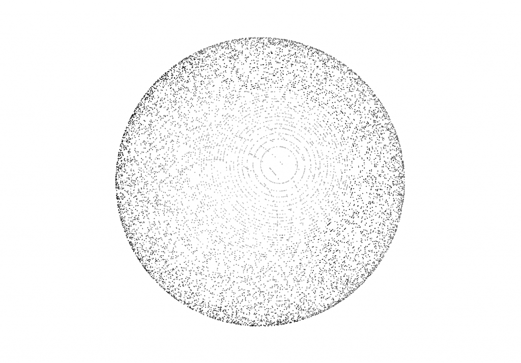
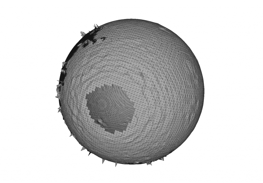
The Moving Least Squares method is popular with users in various domains (medical, geospatial, cultural heritage) because of its resilence towards noisy input and the interpolation between missing data points, leading to the formation of holes with comparable reconstruction approaches. The method has been developed further as Algebraic Point Set Surfaces (APSS)[2] and [Robust] Implicit Moving Least Squares ([R]IMLS)[3]. Examples of their application is shown in the following picture, where a randomly, non-uniformly sampled spherical pointset is reconstructed using MeshLab’s RIMLS implementation. The pointset’s normals are initially approximated using the common kNN approach with N=8. The pointset geometry with normals is then taken as an input to RIMLS with standard parameters. Even though the random sample poses a large challenge to Normal estimation and other reconstruction algorithm, RIMLS reconstructs 2 consistent segments from the input.

Another prime example that shows the application of the least squares optimization was shown by Bruno Levy in 2001 [4], where the method is used in Computer Graphics in the context of Texture Mapping. Here, the objective is, given a global surface parametrization and a mapping function from the object’s parameter space to the image space, and given a set of control points linking both spaces, to derive a global mapping between both spaces. The least squares method is used to minimize the distance between each target texture coordinate and its parameter’s computed value. The gradient is determined by local geometry neighbourhoods. The best overview on how that works can be seen on the website to the method.

A method from the realm of Computer Vision is given by Horn in 1987 [5]. He developes a closed-form solution to the least-squares problem of obtaining absolute orientation values for unit quaternions. Horn uses in his paper the least-squares method to minimize the error between 3D vertex measurements in 2 coordinate systems with matched correspondances. He forms a vertex triad to recover the mutual affine rigid transfomation. Because the selection of different vertex triads delivers different results, a least squares method between all triad combinations is used. The re-transformation error is used to determine subsequently scale, translation and rotation.

CODE EXAMPLE

As an example for coding, I hereby want to introduce a toy example of regression from the realm of photometry. Let’s assume we are given a collection of images, where we want to separate foreground and background, or classify it further (structure, landscape, sky). Although classification usually exploits the sigmoid function, we formulate the approach as such: Taken a collection of sample points that are manually segmented according to the target scheme, can we devise a function that allows us to automatically segment further images ? Turns out: yes, it may be possible.

We need to parametrize our function, for which we use HLS colour values of respective image points. The function formulation is as follows:

, where Y is our vector of expected output segment values and X is a N-by-M matrix (N being the number of point samples, M being the function dimensionality). It is a linear problem formulation having 3 input parameters:

X_0 is our constant model input parameter, here being 1. „a“ is the resulting parameter vector we try to approximate using Least Squares. In the code example, we determine the parameters by solving the Normal equation for the equation system. The code example uses the commonly available Eigen library (libeigen3). The code developed for this example is available at Github.

The referred sample images are taken from flickr’s CC-licensed database. Acknowledgement goes to Tom Hall and Rusty_Clark for the sample images.

The program takes as input an Nx1 m-file with vector Y and an NxM m-file with matrix X, putting out an Mx1 m-file with vector a.

@INPROCEEDINGS{Alexa2001,
author = {Alexa, Marc and Behr, Johannes and Cohen-Or, Daniel and Fleishman,
Shachar and Levin, David and Silva, Claudio T.},
title = {Point Set Surfaces},
booktitle = {Proceedings of the Conference on Visualization '01},
year = {2001},
series = {VIS '01},
pages = {21--28},
address = {Washington, DC, USA},
publisher = {IEEE Computer Society},
acmid = {601673},
isbn = {0-7803-7200-X},
keywords = {3D acquisition, moving least squares, point sample rendering, surface
representation and reconstruction},
location = {San Diego, California},
numpages = {8},
owner = {christian},
timestamp = {2015.06.03},
url = {http://dl.acm.org/citation.cfm?id=601671.601673}
}

[2] G. Guennebaud and M. Gross, „Algebraic point set surfaces,“ Acm trans. graph., vol. 26, iss. 3, 2007.
[Bibtex]

@ARTICLE{Guennebaud2007,
author = {Guennebaud, Ga\"{e}l and Gross, Markus},
title = {Algebraic Point Set Surfaces},
journal = {ACM Trans. Graph.},
year = {2007},
volume = {26},
number = {3},
month = jul,
acmid = {1276406},
address = {New York, NY, USA},
articleno = {23},
doi = {10.1145/1276377.1276406},
issn = {0730-0301},
issue_date = {July 2007},
keywords = {moving least square surfaces, point based graphics, sharp features,
surface representation},
owner = {christian},
publisher = {ACM},
timestamp = {2015.08.06},
url = {http://doi.acm.org/10.1145/1276377.1276406}
}

[3] A. C. Öztireli, G. Guennebaud, and M. Gross, „Feature preserving point set surfaces based on non-linear kernel regression,“ Computer graphics forum, vol. 28, iss. 2, p. 493–501, 2009.
[Bibtex]

@ARTICLE{Oeztireli2009,
author = {\"{O}ztireli, A. C. and Guennebaud, G. and Gross, M.},
title = {Feature Preserving Point Set Surfaces based on Non-Linear Kernel
Regression},
journal = {Computer Graphics Forum},
year = {2009},
volume = {28},
pages = {493--501},
number = {2},
abstract = {Moving least squares (MLS) is a very attractive tool to design effective
meshless surface representations. However, as long as approximations
are performed in a least square sense, the resulting definitions
remain sensitive to outliers, and smooth-out small or sharp features.
In this paper, we address these major issues, and present a novel
point based surface definition combining the simplicity of implicit
MLS surfaces [SOS04,Kol05] with the strength of robust statistics.
To reach this new definition, we review MLS surfaces in terms of
local kernel regression, opening the doors to a vast and well established
literature from which we utilize robust kernel regression. Our novel
representation can handle sparse sampling, generates a continuous
surface better preserving fine details, and can naturally handle
any kind of sharp features with controllable sharpness. Finally,
it combines ease of implementation with performance competing with
other non-robust approaches.},
doi = {10.1111/j.1467-8659.2009.01388.x},
issn = {1467-8659},
keywords = {Point-based reconstruction, robust, implicit moving least squares},
owner = {christian},
publisher = {Blackwell Publishing Ltd},
timestamp = {2015.08.07},
url = {http://dx.doi.org/10.1111/j.1467-8659.2009.01388.x}
}

@INPROCEEDINGS{Levy2001,
author = {Lévy, Bruno},
title = {Constrained Texture Mapping},
booktitle = {ACM SIGGRAPH conference proceedings},
year = {2001},
month = {Aug},
organization = {ACM},
publisher = {Addison Wesley},
owner = {christian},
timestamp = {2015.06.03}
}

@ARTICLE{Horn1987,
author = {Horn, Berthold KP},
title = {Closed-form solution of absolute orientation using unit quaternions},
journal = {JOSA A},
year = {1987},
volume = {4},
pages = {629--642},
number = {4},
owner = {christian},
publisher = {Optical Society of America},
timestamp = {2015.06.03}
}